Our service provider had about 4 hour outage last night due to a disk array failure. The VM for our site was migrated to new hardware and was back online at about 1:30am EST today.
Everything should be working, and signalserver is back running. It’s actually a bit faster on the new hardware.
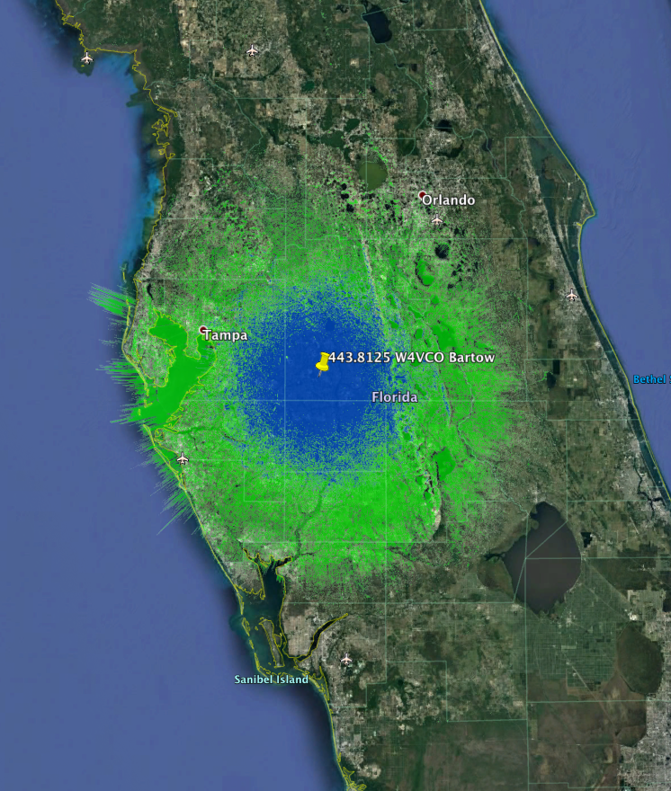
443.8125|448.8125|7K60FXE|NULL|NULL|NULL|1|1|1|2|0|NULL|NULL|NULL|NULL|1485|1|W4VCO|Julian A. Homan, W4VCO|Bartow|2020-01-03|2020-01-03|27.75|-81.89|126.00|LTOWER|455-5N|212|12.500|50|97|NULL|NULL|1|https://plots.fasma.org/440/443.8125_W4VCO_Bartow_1485.kmz|NULL|NULL|NULL|NULL|NULL|NULL|NULL|NULL|NULL|NULL|NULL|0|NULL|1
With the recent success of modeling all coordinated repeaters in the state, we’ve found some issues with the existing data. Issues including, coordinates being way off, powers wrong, ERP wrong and so forht. Then a major problem in northern Florida was discovered, models were ignoring the digital elevation model (DEM) when coverage was being plotted.
FASMA uses an implementation of Longely-Rice or the Irregular Terrain Model which takes into account the elevations of terrain and loss due to signals scattering and absorbed by terrain. Essentially when this data is missing it’s assumed as sea-level and the model generated is very smooth, and concentric about the transmitter. Such a model is quite far off from reality, and can over or under state the coverage (understanding is possible as we assume the antenna height above ground is now at sea level, not the actual height).
The DEM data used was provided by the Shuttle Radar Topography Mission (SRTM) which mapped the surface of the earth at resolutions not available before. The earth was scanned and elevation was averaged over 1 and 3 arc-seconds (30m and 90m). FASMA uses the 90m data as there is little gained, other than a much longer processing time, using the 30m average for non-microwave work. The USGS has several different versions of this data released, but by the most common is 2.1, which has the ability to be directly downloaded from a web-server at the USGS.
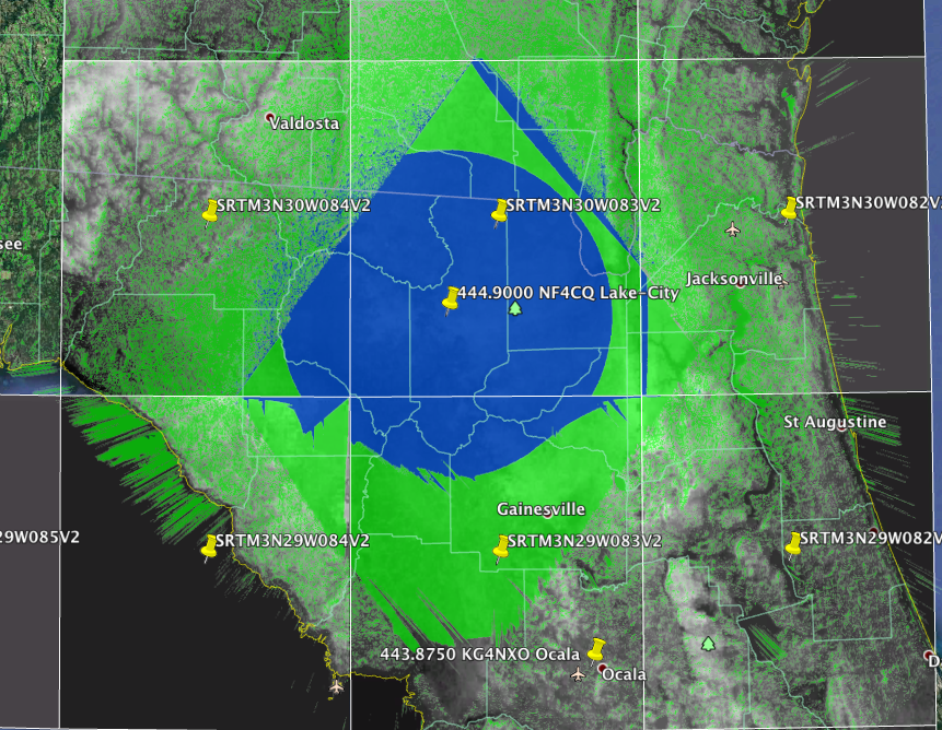
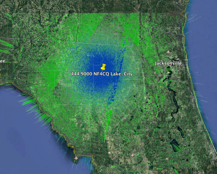
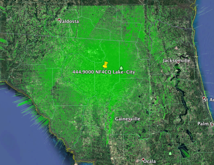
This brings us to the issue with north Florida. An example for this is the below repeater model:
NF4CQ Lake City with bad DEM data
The solid color area here indicates the model has no variation in elevation for most of it. This appears to be a rhombus shaped void centered just south of Lake City and obscuring most of North Florida. The underlying SRTM data was checked and found to possess the same void.
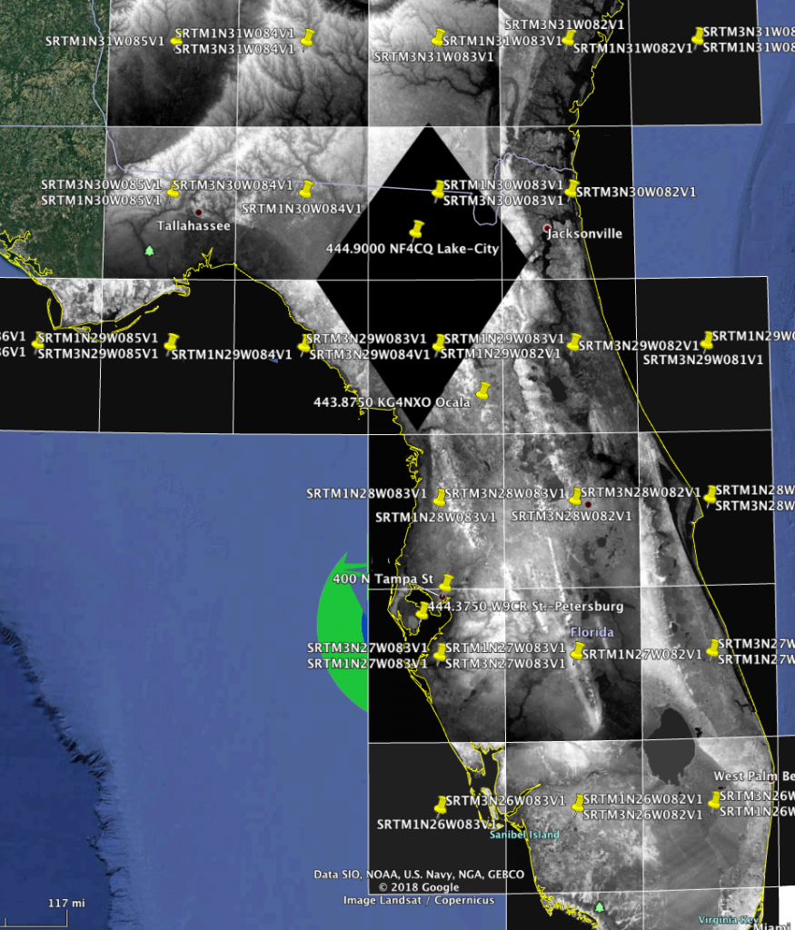
This discovery prompted much research into the SRTM data, and the 30m data was found to have the same issue. In the image below it can be seen of a massive gap across north Florida. Further research found this to be a product of “voids” or gaps in the SRTM radar. Typically this effects areas of deep canyons and high variation where the radar cannot see due to the angle of the shuttle to the surface of the earth. These areas of uncertainty are removed and set to negative elevation.
Black is Sea-Level, note the gap from Ocala to the State Line
USGS has newer versions of data available, known as Version 3 and includes what’s know as void fill, however it is not available for direct download. An account is required and one must point-and-click through the USGS map server interface for it. This precludes downloading automatically, as the number of 3 x 3 tiles required for US coverage is impractical to download by hand. The download is also in a different format than the HGT SRTM standard, and would need to be converted. As luck would have it, there is a web download of the SRTMv3 data as the HGT files, but it requires a user/password once registered with USGS. Using this password and some shell scripting, the entire world was able to be downloaded as SRTMv3 HGT zip files. All 14280 of them.
As the FASMA modeling program is based on SPLAT!, a conversion is required to SDF from HGT of the data. The SDF files are much larger with the entire wold of SDF files taking ~77 GiBytes of space. SPLAT! does support bzip2 compressed SDF, and a multi-threaded version of bzip2, pbzip2 was uses to compress the files in short order on a 24 core server. This compressed down to a more reasonable 10 GB.
After remodeling a number of repeaters in North Florida, it was found some tiles of DEM data looked to be corrupted, with some areas below sea-level and others with “noise” data in them. Comparisons were made with the source SRTM files and found to be perfect. Data looked good and gdal_translate was used to make PNG’s of the terrain, confirming the SRTMv3 was not the source of the issue.
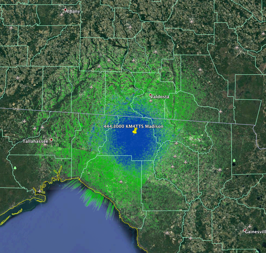
Tile issue with some corruption in this tile at N30W82
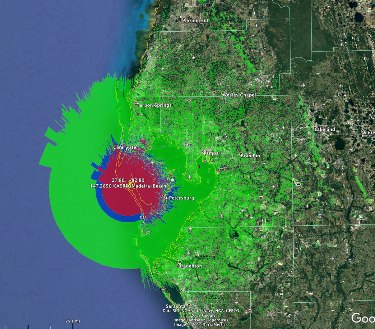
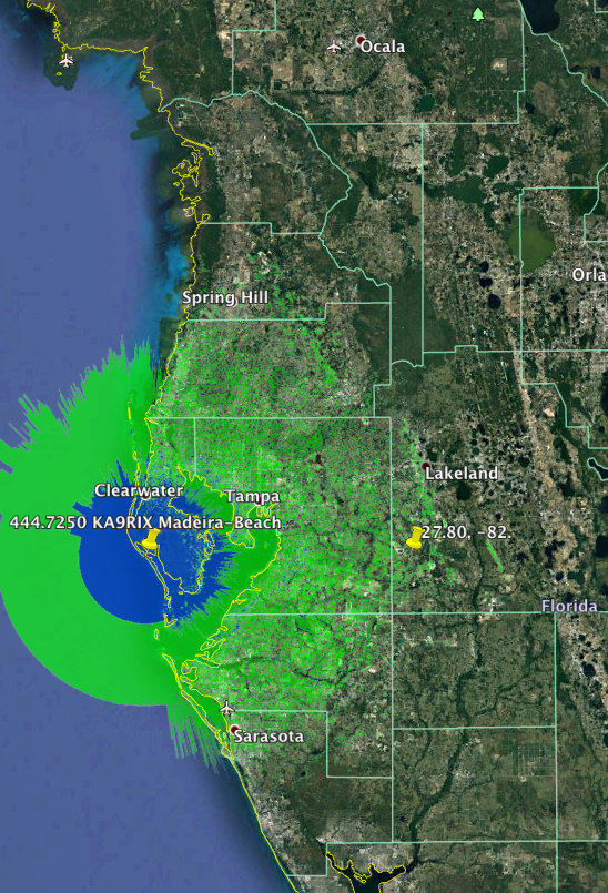
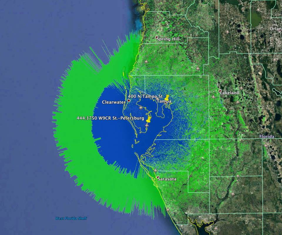
W9CR St Pete repeater with bunk data
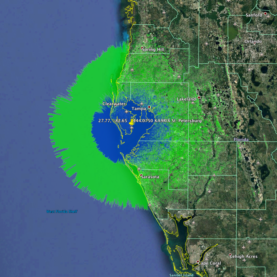
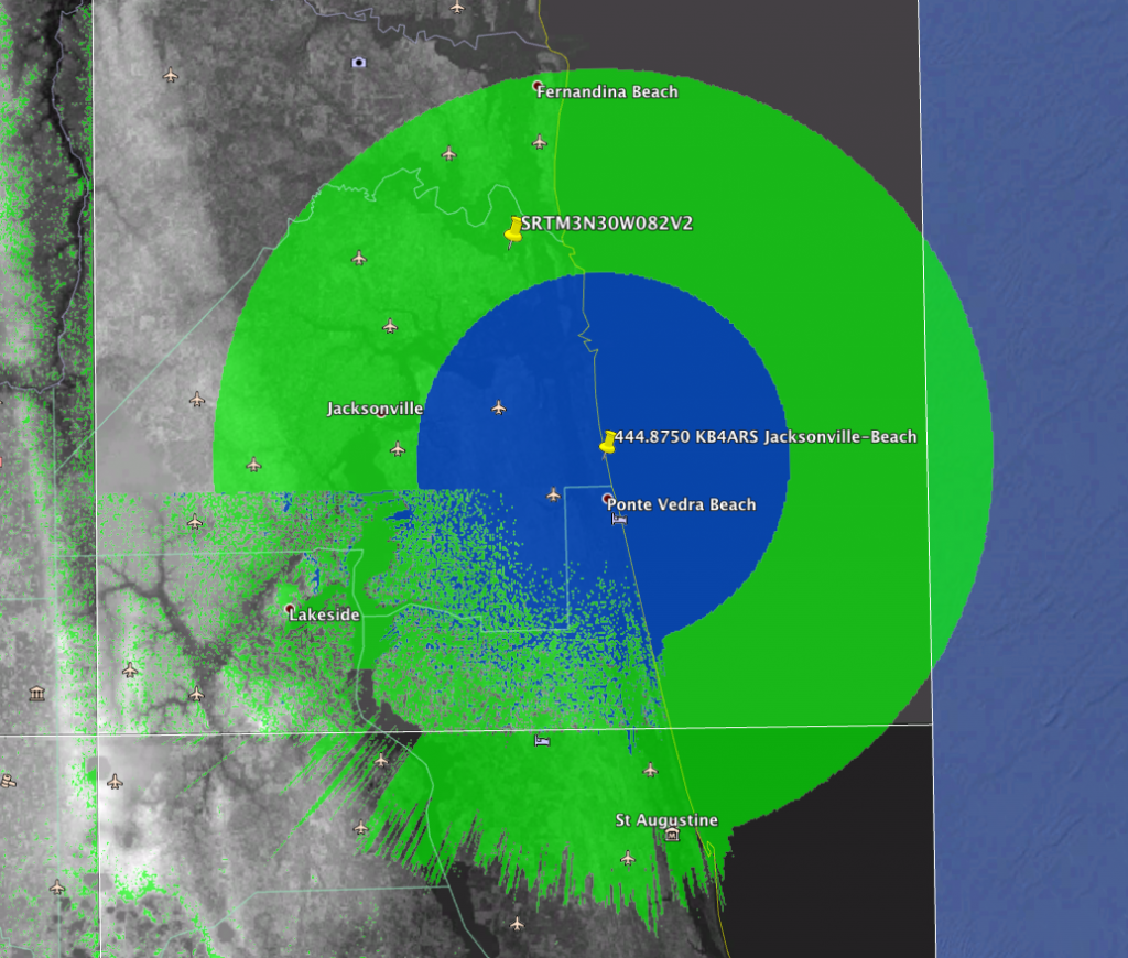
After much trial and error to locate the bug, it was discovered uncompressed SDF files worked fine. Further when compressed again with bzip2, the resulting sdf.bz2 file rendered as expected. This was quickly confirmed as the library in SPLAT! not being able to decompress files compressed with pbzip2 perfectly. A script was made to unbzip and then bzip2 all sdf files in place. The results below show it was a simple fix. The ultimate issue will be submitted as a bug report.
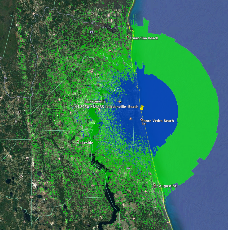
JAX repeater with proper DEM
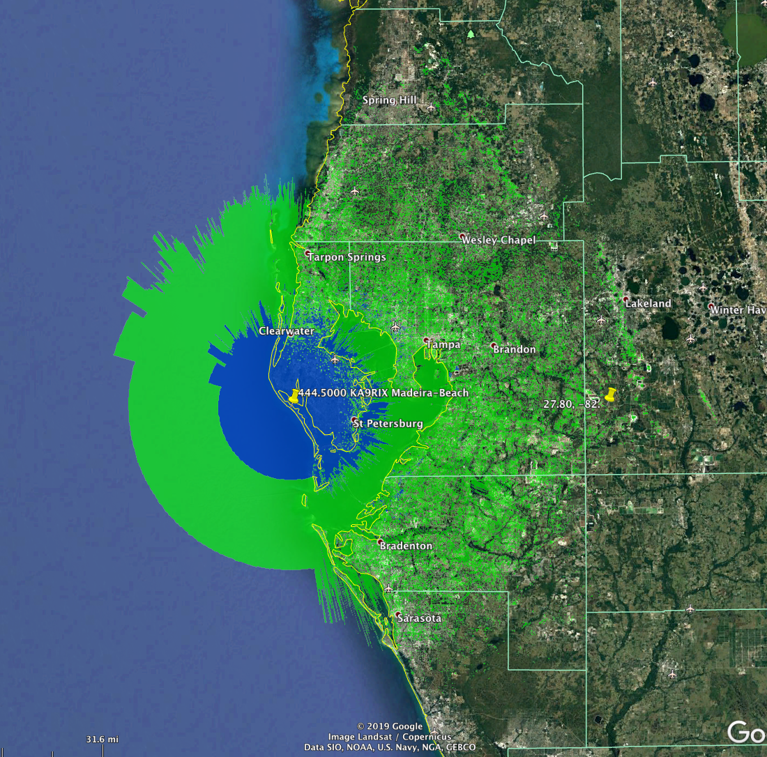
St Pete Repeater fixed
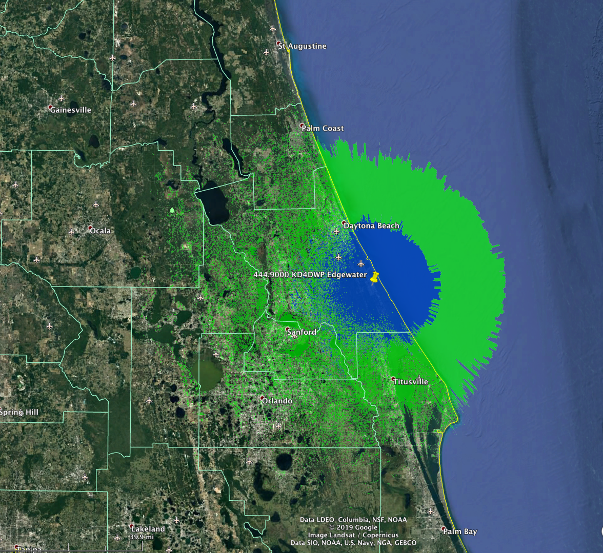
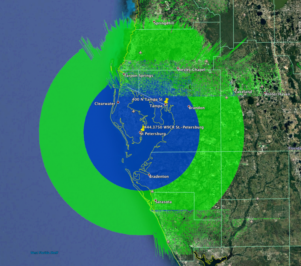
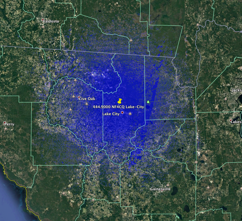
The Lake City 444.9000 NF4CQ revised plots using the SRTMv3 models are below. Note due to the void “fill” it’s not a perfect and we have some discrepancies in the elevation corrections and the valid SRTM data. This is not perfect but it’s much better than assuming sea-level, especially for elevations in North Florida where 30-40m ASL is normal.
Combined
Interference Plot
Service Plot
References:
http://srtm.fasma.org/ – FASMA has made it’s collection of SRTMv3 HGT and SDF data for the wold available for direct download.
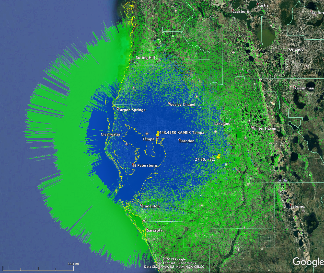
Recently we’ve completed the modeling of all coordinated repeaters in Florida. This was scripted and database driven modeling. Right now the individual KMZ files are available at https://plots.fasma.org under the various bands. Each KMZ file has the service, interference and point of repeater, along with channel size and modulation type.
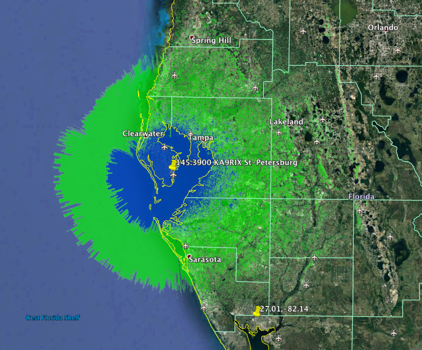
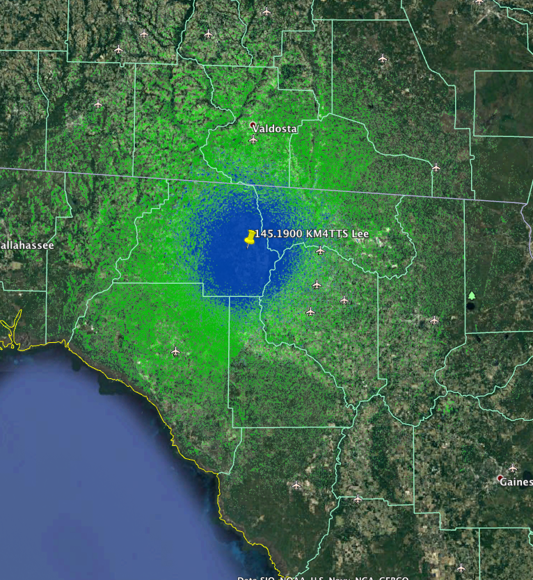
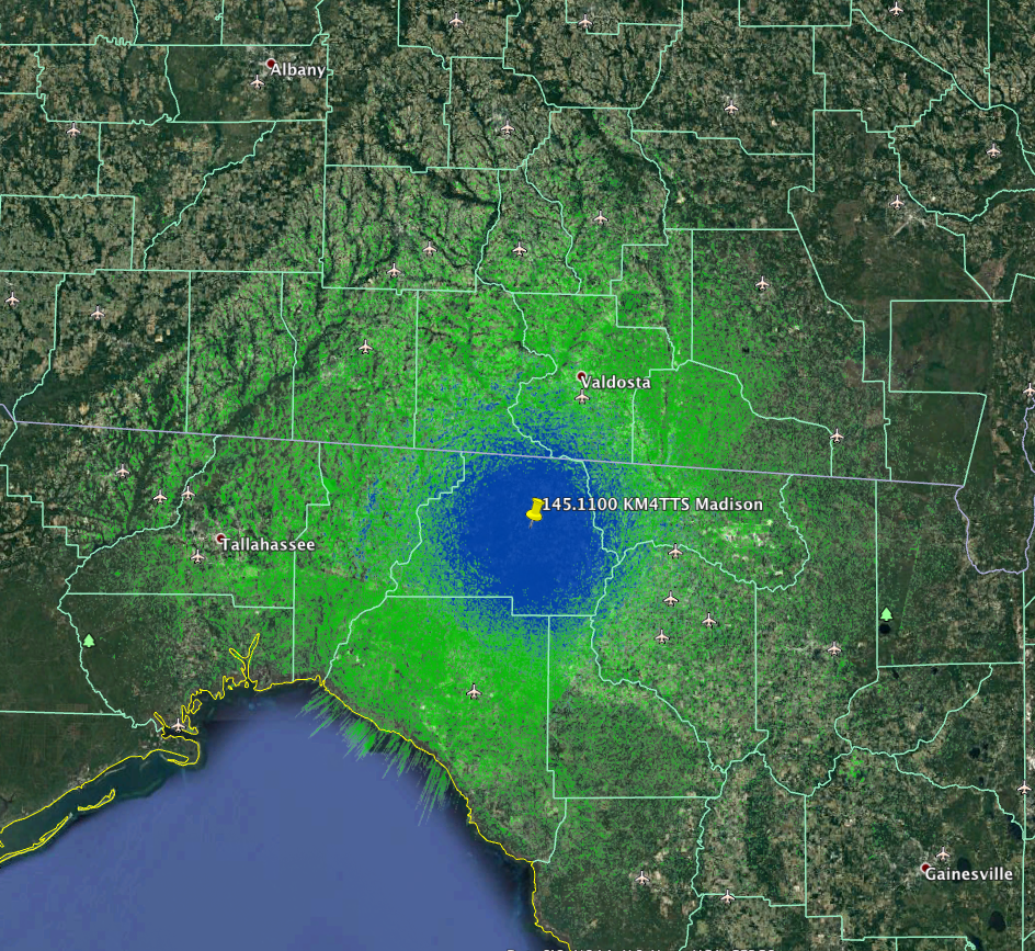
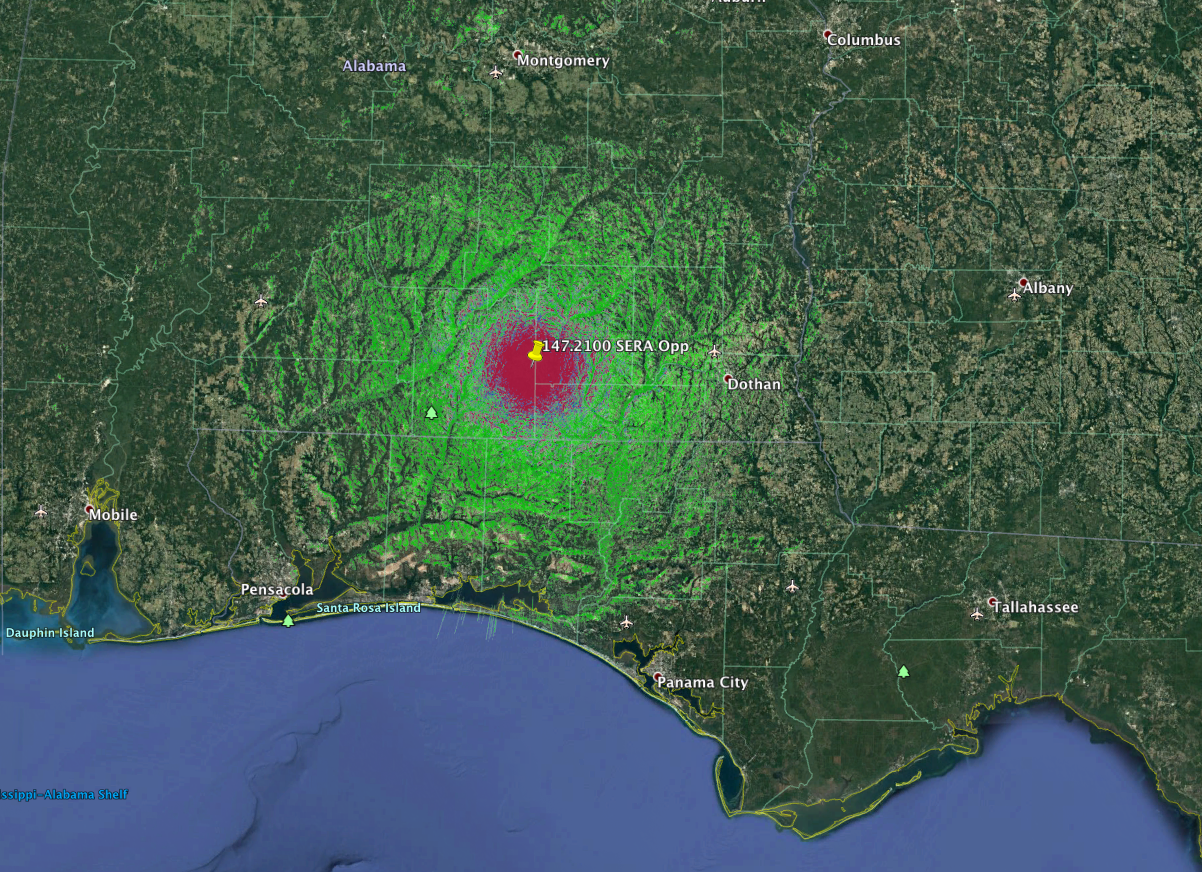
Most repeater owners/operators/trustees will look at the service contour which is in blue. This shows an area where at 1.83m (6′) above the ground, there is a 50% chance that location will have a signal, 50% of the time greater or equal to the service contour. This is typically the mobile service area of a repeater and designated (50, 50).
The green interference contour is modeled to show 50% of locations 10% of the time (50,10) where a signal will be 18 dB below the service contour. This de-rating to 10% makes the chances of receiving a signal much smaller and thus the interference contour is larger. No other co-channel users interference contour should overlap the service contour of any other repeater. This ensures a repeater in it’s protected service contour has a signal at least 18 dB greater than any co-channel repeaters.
In some cases there are adjacent contours, and these are used much like the interference contour. No adjacent contour should overlap another service contour. These are used on 144-146 and 146-148 MHz and for narrowband in 222-225 MHz.
The eventual goal is to have this database driven in real time. This is being worked on and we hope to have a much better interface shortly.